
Click here for the most recent polymath3 research thread. A new thread is comming soon.

Emmanuel Abbe and Erdal Arıkan
This post is authored by Emmanuel Abbe
A new class of codes, called polar codes, recently made a breakthrough in coding theory.
In his seminal work of 1948, Shannon had characterized the highest rate (speed of transmission) at which one could reliably communicate over a discrete memoryless channel (a noise model); he called this limit the capacity of the channel. However, he used a probabilistic method in his proof and left open the problem of reaching this capacity with coding schemes of manageable complexities. In the 90’s, codes were found (turbo codes and LDPC rediscovered) with promising results in that direction. However, mathematical proofs could only be provided for few specific channel cases (pretty much only for the so-called binary erasure channel). In 2008, Erdal Arıkan at Bilkent University invented polar codes, providing a new mathematical framework to solve this problem.
Besides allowing rigorous proofs for coding theorems, an important attribute of polar codes is, in my opinion, that they bring a new perspective on how to handle randomness (beyond the channel coding problem). Indeed, after a couple of years of digestion of Arıkan’s work, it appears that there is a rather general phenomenon underneath the polar coding idea. The technique consist in applying a specific linear transform, constructed from many Kronecker products of a well-chosen small matrix, to a high-dimensional random vector (some assumptions are required on the vector distribution but let’s keep a general framework for now). The polarization phenomenon, if it occurs, then says that the transformed vector can be split into two parts (two groups of components): one of maximal randomness and one of minimal one (nearly deterministic). The polarization terminology comes from this antagonism. We will see below a specific example. But a remarkable point is that the separation procedure as well as the algorithm that reconstructs the original vector from the purely random components have low complexities (nearly linear). On the other hand, it is still an open problem to characterize mathematically if a given component belongs to the random or deterministic part. But there exist tractable algorithms to figure this out accurately.
Let us consider the simplest setting. Let 


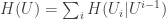


Here 


Also note that defining 


Over the past two years, this result has been extended to random variables valued in 


The original paper is “Channel polarization: a method for constructing capacity-achieving codes for symmetric binary-input memoryless channels“, published in July 2009 in the IEEE Transactions on Information Theory. Arıkan received the IEEE Information Theory best paper award this year. This paper deals with the polarization of `channels’, whereas here I discussed the polarization of `sources’ (less general but same technique).
Emmanuel Abbe, emmanuelabbe@gmail.com
Additional links: historical take on polar codes;
Update (January 15) Here are three lectures by Erdal Arıkan on Polar codes at the Simons Institute.

Pingback: Tweets that mention Emmanuel Abbe: Polar Codes | Combinatorics and more -- Topsy.com
If it is not already obvious from the context: the construction of polar codes is nothing but identifying the coordinates where the entropy polarizes to 1. For the trivial binary erasure channel (for which capacity achieving efficiently encodable-decodable codes were already known) it is a relatively easy task. However, for the other channels, like binary symmetric, a systematic construction is still an open question. Recently Tal and Vardy claimed that they have a construction; no manuscript is available for scrutiny though.
The big advantages of polar codes are: being linear, and formed with the similar structure of Reed-Muller code, they can be easily encoded and decoded, once constructed. Also to be noted, these codes are “asymptotically bad,” their distance is a vanishing proportion of length.
In any way, this is the only true breakthrough in coding theory in at least the past 10 years IMHO. A great paper.
I don’t understand, what was the breakthrough theorem? (or was it a breakthrough approach ?)
A new proof of Shannon’s coding theorem?
A coding scheme which has a near-linear time algorithm for decoding, and which meets Shannon capacity? Wasn’t this achieved by Forney in the 1970s (by concatenation), that too by an explicit code?
Is it that polar codes are “simple” (even though they are not explicit)?
Or is it that once we do make them explicit, they might have better dependence on the parameter epsilon, when you use these codes at rate R = C – epsilon, where C is the capacity?
This confusion might be a result of the difference between theoretical computer science approach to coding theory, and the electrical engineering approach to coding theory.
Sam: It’s not a proof of Shannon’s coding theorem.
The concatenation code of Forney did not reach the capacity with a near linear-time algorithm as far as I remember (when you approach capacity the outer code part start mattering). For any epsilon>0 (as you wrote), polar codes allow an error probability of O(2^{-\sqrt{n}}) (with an exponent in epsilon that is strictly positive) and a complexity of O(n log n) (independent of epsilon and taking into account the procedure that figures out the classification of the indexes). Even if you ask for weaker decays in the error probability, I am not sure that there exist other codes providing such mathematical guarantees. Do you know any? What do you mean by “better dependence”?
In any case, when Gil asked to write on his blog, I thought it would be more interesting/general to put emphasis on the probabilistic phenomenon of polarization (the 0-1 result using the Kronecker structure) rather than the channel coding problem. This is however only one step (although the key one I think) used in the coding scheme of Arikan (see paper). Hope this helps.
This is not a new proof of Shannon’s coding theorem. The breakthrough result is the following “We have efficiently encodable/decodable class of codes that achieves the capacity of symmetric channels, with the given decoding.”
A coding scheme which has a near-linear time algorithm for decoding, and which meets Shannon capacity? Wasn’t this achieved by Forney in the 1970s (by concatenation), that too by an explicit code?
No. Forney’s `explicit’ concatenated codes do not achieve capacity. When you say explicit construction what do you mean? Outer Reed-Solomon codes, I assume; what are the inner codes ? GMD decoding?
Is it that polar codes are “simple” (even though they are not explicit)?
They are simple enough. So far, there is no computational shortcut in construction though, for general symmetric channels.
Or is it that once we do make them explicit, they might have better dependence on the parameter epsilon, when you use these codes at rate R = C – epsilon, where C is the capacity?
The decoding complexity here is independent of such epsilon. I think that is what you have in mind. The decoding probability error is already discussed above.
This confusion might be a result of the difference between theoretical computer science approach to coding theory, and the electrical engineering approach to coding theory.
I think finding capacity achieving codes is one central topic in coding theory, and historically most important; the other problems being bounds on the size of codes (closing the gap), explicit codes that achieves GV bound for all rate etc.
I find the polar codes fascinating from several reasons.
First, given n and p it is a nice mystery which are the bits which carries maximal entropy and which are the bits that carries almost no entropy. In his lecture at Yale, Emmanuel mentioned that this is an open problem and that there are some indication that the indices of the “useful” bits has some fractal nature.
Second, this looks like a very general phenomena and will probably work for other matrices. (Although it will be less useful).
Third, there are various possible analogs. Suppose, for example you replace bits with qubits the Bernouli (p) distribution by some quantum operation (or just a simple depolarizing channel) and the matrix G by a hadamard matrix. I suppose that the polarization phenomena will prevail and this may be useful too.
Forth, the (naked) polarization phenomenon reminds me of the phenomenon of noise synchronization that I studied. (See also this mathoverflow question.)
Actually, it would be useful to indicate how the proof of the polarization property goes. from Emmanuel’s lecture I remember it is quite simple.
Second, this looks like a very general phenomena and will probably work for other matrices. (Although it will be less useful).
This is already done here:
Click to access polar_exponent_journal.pdf
Also discusses the effect of Matrix size on error exponent.
I think that what Gil has in mind regarding
“this looks like a very general phenomena and will probably work for other matrices. (Although it will be less useful)”
is even more general than what has been looked at in the paper you refer to Arya.
The paper you mention considers other choices for the small matrix (the [1 1, 0 1]) which can be of dimension k x k where k is fixed. It characterizes the matrices for which polarization happens (indeed it happens for most matrices). Interestingly, the paper concludes that it is not worth considering anything else than the initial 2×2 matrix: to have any gain in the convergence rate (and error decay), one has to consider k to be at least 16, with a very small improvement with respect to a big cost in complexity and dimensionality growth (n is now a power of 16 now).
However:
1. one may consider matrices which are not of this kronecker form; of course it’s kind of the crux of polarization to have the kronecker structure, but still, the problem of having radical changes between two sets of components may happen in more general settings. Gil may be referring to this?
2. one may keep the kronecker structure and consider non linear mappings, or linear in GF(q). That I think can give interesting results to be analyzed with our current tools.
The definition of conditional entropy depends on the order of the particular index, with a stricter condition on each index as it grows. Does this mean that for simple cases such as p-biased coins, the indices where conditional entropy is one will be the first pn indices? (Intuitively this seems to me to be the case if you take a random matrix instead of Kronecker product.)
Dear Boaz Barak,
Yes I would agree with your intuition for some random matrix ensembles (provided that there is a sharp transition, and I guess you meant H(p)n instead of pn) . Indeed, it would be good to check this.
Gil: have you tried it?
I remember you asking a similar question.
Regarding the Kronecker case, it s a bit different. That s where the fractal-like shape comes in. It is true that at the beginning you see many 1’s (O(n) i guess but no proofs) and at the end you see many 0’s. However in between we don’t quite understand what happens.
For an arbitrary integer between 1 and n, it s hard to predict what happens. It can jump back and forth from o to 1…
First, we want _low_ conditional entropy, since this means _high_ mutual information. So you should reverse your directions.
When computing the transformation (x,y) -> (x+y,y), the second coordinate is indeed much better. That means that for each “1” bit in your index you’re winning, and for each “0” bit you’re losing. But the order matters!
The case of binary erasure channels is worked out in the original paper (it’s pretty easy). If the probability of non-erasure is e, then the original mutual information is e, a 0-bit corresponds to applying x->x^2, and a 1-bit corresponds to applying x->1-(1-x)^2. Figure 4 on page 3 of the paper shows the messy results (though perhaps bit-reversing the indices would have resulted in a nicer graph).
In general, define V_t as the subspace generated by all rows (or columns) but the first t. Let H_t = H(C(v_t)), where C is your channel, and v_t is a random vector from V_t. The mutual information of bit t is H_t – H_{t+1} (unless I made a silly mistake), so the good bits are the ones for which the transition from V_t to V_{t+1} reduces the entropy significantly.
Actually the graph in Arikan’s paper uses the correct bit-order, the other bit-order looks even more erratic.
Nice post!
I have one question: is there any intuitive way to understand this polarization phenomenon?
Gil, Anthony: regarding the proof of the 0/1 result (and maybe some intuition), here is the idea.
Check first what happens when n=2, i.e., we take [X,X’] iid and we map them to [X+X’,X’]. Since G_2 is invertible:
2H[X]=H[X,X’]=H[X+X’,X’]=H[X+X’]+H[X’|X+X’] (*)
(the last equality results from factorizing the distribution of [X+X’,X’].)
We must have H[X’|X+X’]=H[X]. So if you compare what happens before and after the G_2 map, we initially had a random vector with the randomness spread out uniformly, and we have created a new random vector which has a first component that is more random and a second one that is less given the first one.
But the total amount of randomness is the same, it’s just been shuffled.
In a game where you had to guess one component and could query the other one, and you have to choose with which of the 2 random vectors you want to play, you should chose the second one.
Now, the rest of the proof relies on the Kronecker structure. Multiplying an i.i.d. vector with G_n=G_2^{\otimes log(n)} can be done recursively. A good way to represent the output of G_n is with a tree of depth log_2(n). You start with X at the root, and at each level you are using G_2 (if you go up you add an iid copy of yourself and if you go down you don’t do anything). You can check that at the leaves you exactly get the output of G_n. Then you need to track the CONDITIONAL entropies (not the entropies directly). For this, you introduce a random process to simplify the analysis. You start at the root and go up and down with probability 1/2. The probability on the path set is uniform, so that asking that the conditional entropy of a path ends in a given interval is precisely counting the proportions of conditional entropies leaving in this interval. The key step it that the process tracking the conditional entropies in this tree is a martingale, because of (*) . It’s clearly bounded, so it must converge almost surely. Finally, notice that when it converges, you are in a situation where the action of G_2 does not shuffle much the entropy anymore, and it’s easy to check that this happens only if the random variable is deterministic or purely random (given the past), that is with an entropy of 0 or 1!
I will take a look at your noise sync pb.
Pingback: Linkage « The Information Structuralist
Pingback: Asilomar Conference | GPU Enthusiast