
Alex Lubotzky and I are running together a year long course at HU on High Dimensional Expanders. High dimensional expanders are simplical (and more general) cell complexes which generalize expander graphs. The course is taking place in Room 110 of the mathematics building on Tuesdays 10-12. The first four hours were devoted to an introduction to the course that came with a disclaimer that some of the material is new to us as well, with a promise that the course will occasionally turn into a seminar featuring interesting speakers, and with a hope that perhaps we will be able to discover while running the course interesting questions to answer or ask. It will be too difficult for me to follow the entire course over the blog but I would like to devote two posts to the Introduction with some remarks and backgrounds.
A brief introduction.
The introduction included the following four parts.
Introduction to Expanders: Alex briefly described the definition of expanders, their spectral properties, the relation with random walks, the construction of expanders, the construction of Ramanujan graphs, one brief application.
Introduction to high dimensional complexes: I briefly described higher dimensional topological objects and mainly simplicial complexes, and the notions of homology and cohomology.
Introduction to high dimensional expanders: I briefly went over several possible (not equivalent) definitions: Cohomological definition; geometric and topological definitions; spectral definition;
Ramanujan graphs and complexes: Alex briefly described what they are.
In this post we will go over the first three items. The next post will discuss the fourth item, provide credits, references and links, and also discuss examples, connections, potential applications, and questions.
Introduction
1. Expander graphs
1.1 The definition
Let
be a graph on the vertex set
.
–expander if for every set
of vertices,
, the number of edges of
is at least
.
The set of edges 

.
1.2 Spectral relation
We will mainly be interested in the case where 


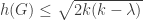
Theorem (Alon-Boppana):

Theorem (Tanner, Alon-Milman):
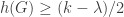
Theorem (Alon):
1.3 Random walks
For regular graphs, the expansion property (through the spectral interpretation) implies that (unless the graph is bipartite) the simple random walk on the graph
We will come back to examples of expander graph and to a certain application after defining high dimensional expansion.
2. High dimensional complexes and homology
We defined abstract simplicial complexes and geometric simplicial complexes 


We described the boundary and coboundary operations. Briefly, if 


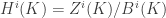
Then we defined the vector spaces – 

Everything we said apply to homology with other fields of coefficients except that it was easier to define the boundary/coboundary operations over Z/2Z (for other fields of coefficients we need to worry about signs). We always consider reduced homology/cohomology without saying it.
3. High dimensional expanders
We mention several different (nonequivalent) notions of high dimensional expansions.
3.1 (co)Homological definition:
Let

Another way to write the same thing is this:
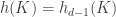
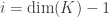
For 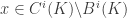

Then 
If 
Some remarks:
1) For graphs: When 


2) 

3.2 Spectral definition
In this little sections we move to chain and cochain groups with real coefficients. Define the Laplacian 
.
Let 

We will say that a 
3.3 Geometric and topological definitions.
Let 


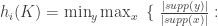
The overlap number w.r.t. 

The topological overlap number of
Note that for graphs, large expansion implies large overlap number.
Next post: Examples, relations between the various definitions, basic research questions. Ramanujan graphs and complexes. Applications: error correcting codes, qantum codes. More remarks, credits and and links to relevant papers.

For a nice account of connections between some of these ideas look at: math.mit.edu/~fox/MAT307-lecture22.pdf
Pingback: Weekly Picks « Mathblogging.org — the Blog
Hi,
is there any chance of the rest of the notes appearing on this blog anytime soon?
Dear Michal, yes I hope so.
Pingback: A High-Dimensional Diameter Problems for Polytopes | Combinatorics and more